TLDR: We make a model valuing draft picks according to how much they outperform their rookie contract (using historical data from 1994-2016). Draft picks tend to be underpaid on the whole (as expected), serving as cheap talent (whereas free agents are ‘properly priced talent’). The most underpaid draft picks are in the late first round and early second round; counterintuitively, this suggests they could actually be worth more than high first round picks.

Originally published on the Brown Sports Analytics blog. Amended below for clarity / brevity.

In March 2017, the Cleveland Browns acquired the maligned Brock Osweiler from the Texans. Osweiler was coming off a disappointing season, and had just signed a massive 4 year, \$72 million dollar contract the year before.

Osweiler was released from the Browns less than six months later, never having played a snap. For his ‘contributions’, the Browns paid \$15.225 million dollars, the remaining guaranteed money on Osweiler’s contract.

Of course, the Browns didn’t want Osweiler - no one did, not with that contract. The only reason the trade happened was because the Texans were willing to pay the Browns to take Osweiler off their hands. The Texans gave the Browns a 2nd round pick, 6th round pick, and Osweiler (with his fat contract), for the Browns’s 4th round pick.

What this boils down to is a draft pick valuation problem. From an asset perspective, the Browns traded \$15.225 million in cap space for a second round pick (minus some change). So, put yourself in the shoes of the Browns braintrust. How would you know if \$15.225 million was a fair price to pay?

In this blog post I will explore a model for valuing NFL draft picks in terms of cap space - and thus implicitly render judgment on the Browns (more on that later). Building a sensible model requires first understanding what we’re modeling - so let’s start there.

Project Overview

Fortunately for us, valuing NFL draft picks becomes a resource management problem - as opposed to a free market-type problem. Vague terminology aside, what I mean is:

• In the NFL, the amount of money a team’s owner has will not really influence how much the team values assets, because each team can only spend up to a fixed salary cap.
• This massively limits the number of variables we have to consider when building the model. For start, the owner’s wealth does not matter. In addition, we do not need to consider outside variables - i.e. whether or not Ronaldo is worth \$100 million depends on the opportunity cost of that \$100 million to the team’s owner, which may be drastically different between owners.
• Finally, in practice, there have been very few instances of NFL owners not willing to spend up to the salary cap. Thus, in building our model we assume we are given the full amount to spend.

This gives us an incredibly controlled optimization problem. Furthermore, every NFL General Manager is essentially trying to solve the same optimization problem. It’s game theory at its finest.

In this optimization problem, we control for just three asset classes: cash, players, and draft capital. Each team is given a set amount of cash (salary cap), and a set number of draft picks each year to begin with. The team must maximize the usage - and accumulation - of these three forms of capital. The hope is that each exchange (money for player, draft pick for player, money for draft pick, etc.) increases the overall value of the assets under the team’s control. If I sign a player “worth” \$8 million for \$4 million, I’ve just increased my ‘asset pile’ by \$4 million. Note this model holds in practice - the 2013 Super Bowl Champion Seahawks paid (in cap space) just over \$18 million for the services of Richard Sherman, Kam Chancellor, Earl Thomas, K.J. Wright, Bobby Wagner, Michael Bennett, Cliff Avril, and Russell Wilson. In an open market, these 8 players would have raked in easily over \$90 million combined per year.

We will use this optimization, ‘asset-pile-building’ framework to develop a model for valuing draft picks.

Model Intuition

The intuition of our draft pick valuation model is as follows:

1. The contract each draft pick receives is fixed in both length and salary (length is generally 4 years, salary depends on how high the selection was), due to stipulations in the NFL’s Collective Bargaining Agreement.

2. Remember our ‘asset pile’ analogy. A draft pick is valuable solely because a drafted player is expected to significantly outperform their contract. In contrast, consider free agency, where any player acquisition is expected to return market value (as NFL free agency is a free market).

   Put another way, no team has an inherent edge in free agency. That doesn’t mean there isn’t strategy, just that generally speaking due to market forces, signing a player in free agency will not tend to grow your asset pile.

3. We first develop a model that determines how much a player deserves to be paid based on how much they contribute. We measure contribution using an existing metric called Approximate Value (AV) - more on AV later. We call a player’s deserved pay fair salary.

4. We then use historical data to determine how much each draft pick number (1st overall, 22nd, 34th, etc.) contributes on average in terms of AV, and convert it to fair salary.

5. We compare each draft pick’s fair salary to their actual salary. The amount the ‘fair salary’ exceeds the ‘actual salary’ is defined as the value of the draft pick. We call this value a draft pick’s surplus.

Surplus

This is a good segue into a key assumption our model makes.

1. The value of a draft pick is equal to its absolute surplus, defined as (fair salary) – (actual salary).

   Example: The first overall pick, by rule, signs a 4 year, \$30 million rookie contract (made up numbers). The fair salary for the first overall pick is \$40 million over four years. The surplus of the first overall pick is $10 million.

   An argument could be made that valuation should be instead percentage return, and not surplus: $$\text{percentage return = }\dfrac{\text{fair value} – \text{actual value}}{\text{actual value}}$$So in the previous example, the percentage return is $\dfrac{1}{3}$.

   However, keep in mind the end goal is the maximize our asset pile. A higher percentage return is obviously preferable if it can be applied to the same amount of capital, but when valuing draft picks, we must perform comparisons where the return is on different, fixed amounts of cpaital.

   For instance, suppose Pick A is paid \$20 million, and has a fair value of \$30 million. Pick B is paid \$10 million and has a fair value of \$18 million. Pick A has a higher surplus, while Pick B has a higher percentage return. You’re offered a choice between the two. Which do you pick?

   If you choose Pick B, you’re getting 80% return on \$10 million dollars, but you’re getting 0% return on the ‘remaining’ \$10 million from Pick A. In other words, I contend that it is more accurate, for the purposes of comparison, to view Pick B as an asset that nets you \$28 million (80% return on \$10 million, 0% return on \$10 million) in return for \$20 million - which is then clearly inferior to Pick A.

Data

Data in this project was scraped using Python’s Beautiful Soup Library as follows:

• AV Data: Scraped from Pro Football Reference
• Player Draft Data: Scraped from Pro Football Reference
• Player Salary Data: Scraped from Spotrac

All data is from 1994 to present (2016), as 1994 was the first year with a salary cap (which our model requires as a key restraint).

Fair Salary

To start, we needed to develop a metric for the ‘fair salary’ for a player - this is defined as the ‘maximum’ salary that a team should be willing to pay for a player in a non edge-case situation (i.e. for instance, one edge case is when a team is far below the minimum spending threshold, and then ‘overspending’ is preferable to having unspent money go wasted).

The premise behind our fair salary metric is that the salary ratio between Player A and Player B should be equal to their contribution ratio. We use Approximate Value (AV) as a proxy for talent and contribution level; Approximate Value is a metric developed by Pro Football Reference designed to measure contribution, and is comparable across positions. It is measured on a yearly basis and is useful as an objective, comparable metric for how much a player contributed to their team in a given year. Read more here.

In making our fair salary metric, we make the following assumptions:

• AV contribution is linear. In other words, a player whose AV is 8 in a given year is worth twice as much as a player whose AV is 4 in a given year.
• A player with 0 AV is worth $0
• A practice squad player’s pay is negligible

Using these three assumptions, we calculate the fair salary for any given player in any given year, using the following formula:

• Let $P$ be that player’s AV in that year.
• Let $SC$ = total combined salary cap across all 32 teams for that year (i.e. 167 million times 32 for 2017)
• Let $N$ = total number of players who can be on an NFL roster in that year (i.e. 53 times 32 for 2017)
• Let $AVTotal$ = Summed AV of the top $N$ NFL players in that year

Then Fair Salary is: $$\dfrac{P}{AVTotal}\cdot SC$$Some of our findings included:

• Matt Ryan, the player with the highest AV in 2016 (also the league MVP), had a fair salary of $16.13 million in 2016.

• The most overpaid player (using ‘cap hit’ as salary metric), in total dollars (not in percentage of salary cap) between 1994 and 2016 was Tony Romo in 2016, whose fair salary was 0, but whose cap hit was over 20 million.

• The most underpaid player (using ‘cap hit’ again as salary metric), in total dollars (not in percentage of salary cap) between 1994 and 2016 was Dak Prescott, whose fair salary was 12.3 million, and whose cap hit was 546,000.

These findings are interesting, but undervalue backups - i.e. some backups have 0 AV but are worth over $0 (i.e. backup quarterbacks).

Draft Pick Historic Performance

Next, for each pick number, we took all the players taken with that pick number from 1994 to 2016, and averaged the annual AV per year over the first four years of those players’ careers (length of rookie contract, fifth year option for first rounders not withstanding).

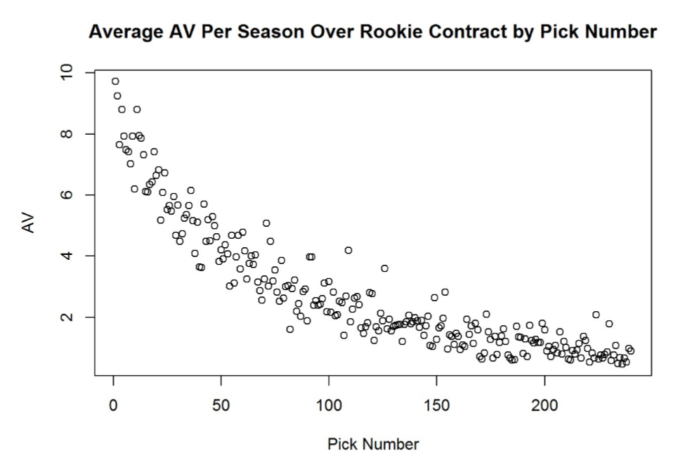
We smooth our data by fitting it to a logarithmic regression. We get the following regression formula, with $R^2 = 0.8676$: $$AV = 7.07347 e^{-0.0099652 * [\text{pick number}]}$$

Calculating Fair Salary for Draft Picks

We now have a function representing the expected AV contributions for each pick number, which we want to convert to fair salary. Let’s calculate the fair salary for draft picks in the 2017 NFL Draft. We make the following assumptions:

1. The salary cap stays the same over the next four years – \$167,000,000. So, $SC$ = 167 million times 32.

2. The NFL roster size stays at 53 and the number of teams stays at 32. So $N$ = 53 times 32.

3. The total AV in all of the next four years is approximated by the average total AV over the last five years (2012 - 2016), which comes out to 6559.

Assumptions #1 and #3 will almost certainly not be true. For assumption #1, knowing that the salary cap will likely increase, we can circle back later and note that our fair salary assumptions are probably conservative. For assumption #3, this value stays relatively constant over the years, so we are fairly confident any differences will be marginal. Our results come out…

Calculating Surplus

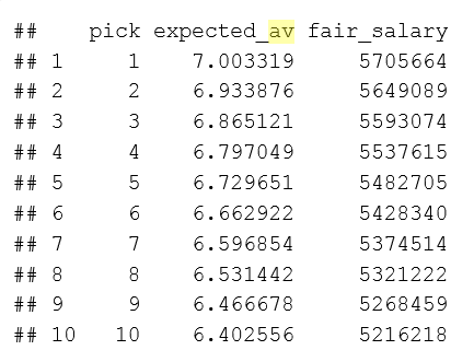
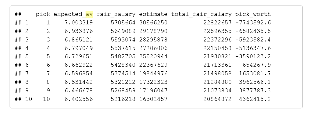
Finally, the part we’ve been waiting for! Comparing fair salary to actual salary, we get the following results, where:

• Pick refers to pick number.
• expected_av is the output of the logarithmic regression function from Part Two, for the given pick number.
• fair_salary is the fair salary computed given the expected_av (see Part Three)
• estimate is Spotrac’s salary estimate (summed for all four years) for each 2017 draft pick
• total_fair_salary is the fair_salary times four
• pick_worth is the surplus of the pick (over the entire rookie contract, not annua­­­­­­­­­­lly)

Results and Discussion

In trading for Brock Osweiler this past Spring, the Browns essentially traded \$15 million dollars for a second round draft pick. According to our model, an average second round draft pick provides just \$8 million dollars in surplus, over all four years of the rookie contract.

This means the Browns in essence removed \$15 million from their asset mountain, and only received \$8 million in return.

So, does that mean the Browns made a bad trade? Not necessarily – one explanation is that the Browns wanted to give up present value for future value. In addition, there are intangible considerations - perhaps the Browns wanted more youth in the locker room.

Other interesting takeaways:

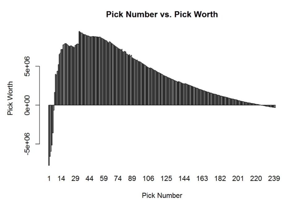
• Our results confirm the idea that draft picks tend to be underpaid.
• High first round picks tend to be overpaid, and under our model, the top six picks in the draft, if made, actually expect to provide negative surplus. In other words, our model is saying teams picking in the top six should actually pass on their pick (remember, each draft pick is actually an option)!
• The most underpaid pick (with the highest surplus) is pick number 33, at the top of the second round. As a General Manager, this also means that trading down in the first round is generally a great strategy.
• The draft is meant in some ways to instill parity in the NFL – the better the team, the worse the pick. If the NFL really wants to institute parity, it should consider reducing the salaries of high first round picks further – as of now, good teams have the advantage in the first round, as late first round picks grow the ‘gold mountain’ more than early first round picks!

These are impactful and meaningful insights, and provide promise for future work. However, we note the following limitations (which we could also address in future work):

• The fifth year option for first round picks is not factored into the valuation. For first round picks, teams get a ‘option’ to add an additional fifth year to the player’s contract, usually at a more expensive salary than the previous four years. For players selected in the first round of the 2014 NFL draft, 23 of the 32 fifth year options were picked up. Thus, we can expect first round picks to be worth slightly more than what our model suggests. Quantifying this would be a worthy next step.
• As aforementioned, another flaw in our model is that we did not account for possible increases in salary cap. The salary cap has increased substantially over the past 23 years, and it is reasonable to expect it to continue to increase. Accounting for this would increase the ‘fair salary’ for the draft picks, and further increase the ‘worth’ of each draft pick. This means that our current estimates for pick worth are almost certainly conservative.
• We estimated fair salary by assuming a linear relationship between AV and salary. We lacked a strong basis in making this assumption, and it’s worth testing to see if it’s real or not. A better option might just be to use market data – see the part about Brian Burke’s project in the Important Notes section below.
• Finally, it is important to note that Approximate Value is just as its name indicates, an ‘approximate’ value of a player’s contribution. Creating a better metric could be a sizeable undertaking but would potentially improve results.

A final caveat to note is that these draft pick valuations are only valid for future, unknown draft picks. During the actual draft, these picks should be instead valued based the players available at each selection (which, of course, is not known until usually a few picks before).

Notes and Credits:

1. Well after completing this project, I became aware of a similar project completed by Brian Burke of Advanced Football Analytics in January 2016. Burke’s project also uses AV as a measure of performance and salary cap ‘surplus’ as a measure of NFL Draft pick value. I borrow Burke’s ‘surplus’ term in my writeup – the concept seems useful enough to warrant a custom term. In terms of differences between my project and Burke’s, I calculate projected draft pick performance a bit differently (focusing on first four years of contract) and ‘fair salary’ differently as well (Burke used market data -what a player with a given AV is typically paid - while I calculated fair salary based on a linear model between AV and salary).

2. I also want to give credit to Cade Massey and Richard Thaler, who as Burke mentions in his writeup, produced a landmark paper in 2005 valuing NFL draft picks using a ‘surplus model’ – given that it was a ‘landmark’ paper, I assume that they were the first to use the ‘surplus’ model as relates to the NFL Draft.

3. This was part of a group project in Brown University’s CS1951a Data Science course. My partners were Edan Eingal ’18, Isaiah Bryant ’18, and Kevin Li’ 18. This was my particular ‘part’ of the project, so the ideas, work, and writeup here are largely mine, but I must give credit to Edan for helping scrape some of the data used and managing a SQL database of all the data (he is considered a ‘SQL God’ by some). See more of our group project here.